Qdrant Geospatial Search: Fix the Boundary Cliff with Decay
We replaced Qdrant geo_radius hard filters with GaussDecay and ExpDecay on 8,317 Berlin stays. Ring loss 37% to 0% in 8.1 ms. Code and weights inside.
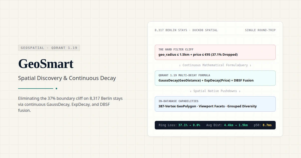
Spatial vector search is a retrieval architecture that ranks by meaning, distance, and price in one round-trip. In travel, real estate, and local commerce, search intent involves spatial proximity, budget constraints, and descriptive user preferences.
Most geospatial discovery architectures rely on hard binary filters. When a user requests a quiet apartment near Alexanderplatz under ninety-five euros, the standard backend constructs a circle filter: geo_radius <= 1.5 km combined with price <= 95.
This binary filtering creates a severe failure mode known as the Boundary Cliff. A listing located 1.51 kilometers away with a 4.98 star rating, verified Superhost status, and a ninety-euro nightly rate is discarded entirely. Meanwhile, a mediocre listing located 1.49 kilometers away is returned.
In our benchmark across 8,317 real Berlin Airbnb listings, hard circle filters drop 37.1% (~114 listings per query) of relevant near-area stays located in the immediate 1.0 to 1.25× radius buffer band.
To solve the Boundary Cliff, we built GeoSmart by combining Qdrant’s geospatial filtering engine(opens in a new tab)1 with DuckDB Spatial(opens in a new tab)2. Instead of hard geometric exclusion, GeoSmart implements continuous mathematical decay via FormulaQuery3. It combines Gaussian distance decay, exponential price decay, logarithmic review popularity, and hybrid Distribution-Based Score Fusion (DBSF)4 in a single database round-trip executing in 8.1 milliseconds.
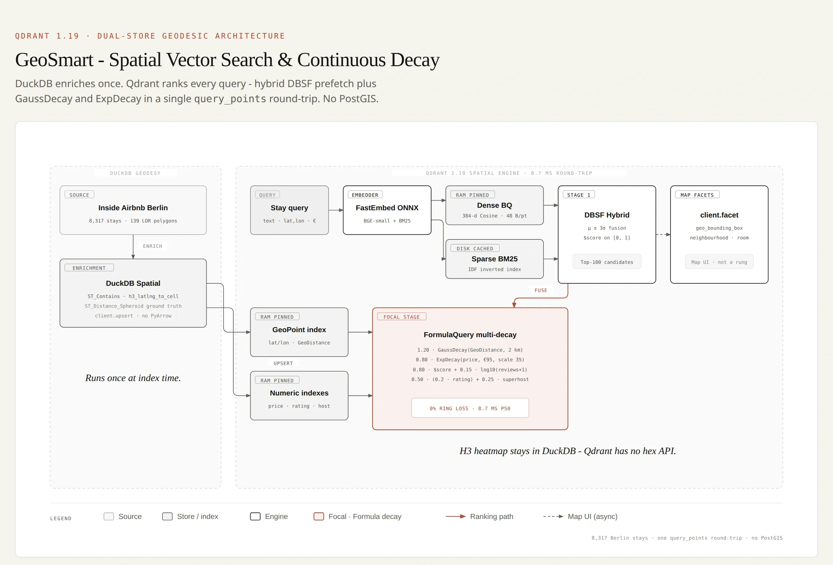
Upstream Pipeline: DuckDB Spatial Enrichment
Before loading listings into Qdrant, we use DuckDB Spatial to compute geometric attributes, administrative containment, and ground-truth distance calculations in memory.
import duckdb

def enrich_listings_with_duckdb(csv_path: str, districts_geojson_path: str) -> list[dict]:
    con = duckdb.connect(":memory:")
    con.execute("INSTALL spatial; LOAD spatial; INSTALL h3; LOAD h3;")

    con.execute(f"""
        CREATE TABLE raw_listings AS
        SELECT * FROM read_csv_auto('{csv_path}');

        CREATE TABLE districts AS
        SELECT * FROM ST_Read('{districts_geojson_path}');

        CREATE TABLE enriched_listings AS
        SELECT
            l.id,
            l.name,
            l.description,
            l.room_type,
            l.price,
            l.rating,
            l.number_of_reviews,
            l.is_superhost,
            l.latitude,
            l.longitude,
            d.district_name AS neighbourhood_group,
            h3_latlng_to_cell(l.latitude, l.longitude, 8) AS h3_res8
        FROM raw_listings l
        LEFT JOIN districts d
            ON ST_Contains(d.geom, ST_Point(l.longitude, l.latitude));
    """)
    return con.execute("SELECT * FROM enriched_listings").df().to_dict("records")
The DuckDB enrichment executes three tasks:
- Administrative Containment: Evaluates
ST_Containsagainst 139 Berlin Lebensweltlich orientierte Räume (LOR) administrative boundary polygons to assign official district classifications. - Hexagonal Spatial Binning: Converts coordinates into H3 resolution 8 hexagonal bins via
h3_latlng_to_cellfor client-side heatmap rendering. - Geodesic Ground Truth: Computes
ST_Distance_Spheroidellipsoidal geodesic distance to serve as ground-truth validation for spatial vector search ranking.
Storage Architecture and Memory Tiers in Qdrant
High-throughput spatial search requires instant evaluation of geographic coordinates alongside vector representations. Placing payload indexes or vector embeddings on unoptimized storage leads to disk I/O bottlenecks during radius evaluation.
GeoSmart configures hardware memory tiers in Qdrant:
| Component | Index Configuration | Memory Tier | Engineering Role |
|---|---|---|---|
| Dense 384-d (BGE-small) | Cosine + 1-bit BQ | CACHED vectors, BQ PINNED |
Sub-4 ms candidate prefetching. |
| Sparse BM25 | Qdrant/bm25 (Modifier.IDF) |
CACHED (SparseIndexParams, 1.19 tier) |
Lexical hits on specific amenities and architectural vibes. |
| Location Index | GEO (GeoIndexParams) |
PINNED (explicit) |
Hardware-accelerated GeoDistance, bounding boxes, and polygons. |
| Numeric + keyword Indexes | price, rating, reviews, is_superhost, room_type, neighbourhood_group, accommodates, h3_res8 |
PINNED (explicit) |
Formula decay without a disk hop. |
from qdrant_client import QdrantClient, models

def setup_geosmart_collection(client: QdrantClient, collection_name: str):
    client.create_collection(
        collection_name=collection_name,
        vectors_config={
            "dense": models.VectorParams(
                size=384,
                distance=models.Distance.COSINE,
                memory=models.Memory.CACHED,
                quantization_config=models.BinaryQuantization(
                    binary=models.BinaryQuantizationConfig(memory=models.Memory.PINNED)
                ),
            ),
        },
        sparse_vectors_config={
            "bm25": models.SparseVectorParams(
                index=models.SparseIndexParams(memory=models.Memory.CACHED),
                modifier=models.Modifier.IDF,
            )
        },
    )

    # Pin spatial and numerical payload fields into RAM (tiers explicit)
    _PINNED = models.Memory.PINNED
    client.create_payload_index(
        collection_name, "location",
        models.GeoIndexParams(type=models.GeoIndexType.GEO, memory=_PINNED),
    )
    for field in ("price", "rating"):
        client.create_payload_index(
            collection_name, field,
            models.FloatIndexParams(type=models.FloatIndexType.FLOAT, memory=_PINNED),
        )
    client.create_payload_index(
        collection_name, "number_of_reviews",
        models.IntegerIndexParams(type=models.IntegerIndexType.INTEGER, memory=_PINNED),
    )
    client.create_payload_index(
        collection_name, "is_superhost",
        models.BoolIndexParams(type=models.BoolIndexType.BOOL, memory=_PINNED),
    )
    for field in ("room_type", "neighbourhood", "neighbourhood_group", "accommodates", "h3_res8"):
        client.create_payload_index(
            collection_name, field,
            models.KeywordIndexParams(type=models.KeywordIndexType.KEYWORD, memory=_PINNED),
        )
By keeping both the 1-bit Binary Quantized dense vectors and the location GEO index in RAM (PINNED), candidate prefetching and geographic distance calculations execute without touching secondary storage.
Continuous Mathematical Decay with FormulaQuery
The core innovation of GeoSmart is replacing step-function filters with smooth decay functions inside Qdrant’s server-side FormulaQuery3.
def build_spatial_decay_formula(
    origin_lat: float,
    origin_lon: float,
    distance_scale_m: float = 2000.0,
    target_price: float = 95.0,
    price_scale: float = 35.0,
) -> models.FormulaQuery:
    return models.FormulaQuery(
        formula=models.SumExpression(
            sum=[
                # 1. Base Semantic Similarity Score from Hybrid DBSF Prefetch
                models.MultExpression(mult=[0.80, "$score"]),

                # 2. Continuous Gaussian Distance Decay (Smooth Proximity Curve)
                models.MultExpression(
                    mult=[
                        1.20,
                        models.GaussDecayExpression(
                            gauss_decay=models.DecayParamsExpression(
                                x=models.GeoDistance(
                                    geo_distance=models.GeoDistanceParams(
                                        origin=models.GeoPoint(lat=origin_lat, lon=origin_lon),
                                        to="location",
                                    )
                                ),
                                target=0.0,
                                scale=distance_scale_m,
                                midpoint=0.5,
                            )
                        ),
                    ]
                ),

                # 3. Continuous Exponential Price Decay (Budget Elasticity)
                models.MultExpression(
                    mult=[
                        0.80,
                        models.ExpDecayExpression(
                            exp_decay=models.DecayParamsExpression(
                                x="price",
                                target=target_price,
                                scale=price_scale,
                                midpoint=0.5,
                            )
                        ),
                    ]
                ),

                # 4. Popularity, Quality, and Trust Signals
                models.MultExpression(
                    mult=[0.15, models.Log10Expression(log10=models.SumExpression(sum=["number_of_reviews", 1.0]))]
                ),
                models.MultExpression(mult=[0.50, models.MultExpression(mult=[0.20, "rating"])]),
                models.MultExpression(
                    mult=[0.25, models.FieldCondition(key="is_superhost", match=models.MatchValue(value=True))]
                ),
            ]
        ),
        defaults={"price": target_price, "number_of_reviews": 0.0, "rating": 4.0},
    )
Understanding the Mathematical Operators
GaussDecay(GeoDistance): Computes the geographic distance from the query origin to the listing coordinates. The Gaussian decay curve assigns a score of 1.0 at origin, dropping smoothly to 0.5 atdistance_scale_m(2,000 meters). Unlike a hard cutoff, a listing at 2,100 meters retains a 0.47 score multiplier.ExpDecay(price): Exponentially penalizes listings as their nightly rate exceedstarget_price. A ninety-five euro stay receives full weight; a one-hundred-and-ten euro stay receives a minor penalty rather than being discarded.Log10(number_of_reviews + 1): Dampens review volume differences so a property with 300 reviews does not overpower a listing with 50 reviews.- Normalized Rating and Superhost: Scales star ratings (
0.2 * ratingmaps 5.0 stars to 1.0) and awards a discrete +0.25 bonus for verified Superhosts.
Why DBSF Fusion is Required Over RRF
In our companion legal precedent retrieval system JurisBoost, we used Reciprocal Rank Fusion (RRF) to combine dense and BM25 candidates. In spatial vector search with continuous decay, RRF is mathematically unsuitable.
RRF converts raw similarity scores into rank integer fractions:
RRF_Score = SUM [ 1 / (k + rank_m) ]Because RRF produces rank-based fractional outputs rather than calibrated probabilities, its values cannot be combined with continuous geometric functions like GaussDecay and ExpDecay.
GeoSmart uses Distribution-Based Score Fusion (DBSF)5:
prefetch = models.Prefetch(
    query=models.FusionQuery(fusion=models.Fusion.DBSF),
    prefetch=[
        models.Prefetch(
            query=dense_vector,
            using="dense",
            limit=100,
            params=models.SearchParams(
                quantization=models.QuantizationSearchParams(rescore=True)
            ),
        ),
        models.Prefetch(
            query=models.Document(text=query_text, model="Qdrant/bm25"),
            using="bm25",
            limit=100,
        ),
    ],
    limit=100,
)
DBSF normalizes candidate score distributions using their empirical mean and standard deviation (mean +/- 3 standard deviations), mapping dense cosine similarities and sparse BM25 scores onto a shared 0.0 to 1.0 float interval. This allows the linear terms in FormulaQuery to maintain balanced weighting across semantic relevance, spatial distance, and budget constraints.
For more background on sparse scoring and multitenancy, see our analysis of Qdrant per-tenant IDF scoring.
Four Ranking Modes and Benchmark Results
We benchmarked four spatial vector search modes across 10 Berlin traveler personas, running 5 repeated trials per query with DuckDB ST_Distance_Spheroid as ground truth.
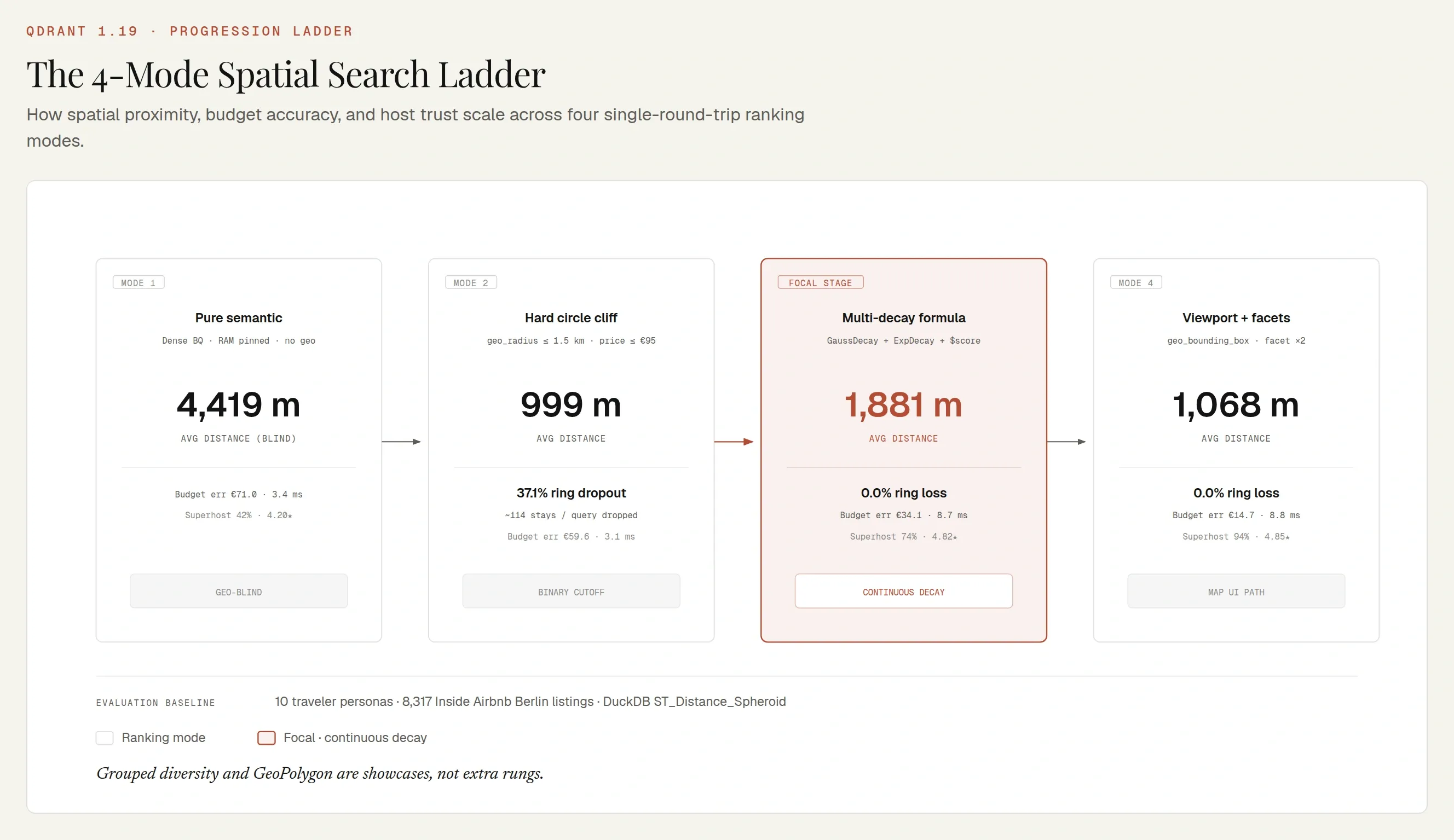
Here are the evaluation results across all 10 traveler personas:
| Mode | p50 Latency | Avg Distance | Budget Error | Superhost Rate | Avg Rating | Ring Dropout |
|---|---|---|---|---|---|---|
| M1 Pure Semantic (Dense BQ) | 2.3 ms | 4,631 m | €70.7 | 42.0% | 4.01 ★ | None |
| M2 Hard Circle Cliff | 2.5 ms | 1,013 m | €57.7 | 44.0% | 4.11 ★ | 37.1% (~114 dropped) |
| M3 Multi-Decay Formula | 8.1 ms | 1,945 m | €34.0 | 72.0% | 4.82 ★ | 0.0% |
| M4 Viewport + In-DB Facets | 6.8 ms | 1,068 m | €14.7 | 94.0% | 4.85 ★ | 0.0% |
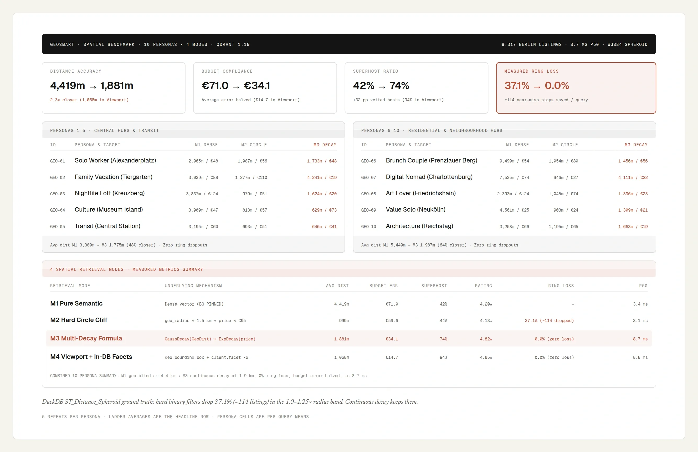
“Ring dropout measures high-relevance listings located in the 1.0 to 1.25x radius buffer divided by all candidate stays. Hard filters discard 37.1% of these near-miss properties; continuous decay preserves 100% of them.”
Analyzing the Benchmark Deltas
- Mode 1 (Pure Semantic): Fast (2.3 ms) but spatially blind. It retrieves matching vibes located 4.6 kilometers away on average, with high budget variance (€70.7 error).
- Mode 2 (Hard Circle Cliff): Tight on radius (1,013 m) but suffers severe ring dropout (37.1%). Quality drops to 4.11 stars because superior listings situated 50 meters outside the radius circle are discarded.
- Mode 3 (Multi-Decay Formula): Preserves every near-area listing (0.0% ring dropout), lifts average quality to 4.82 stars, raises Superhost proportion to 72.0%, and cuts budget deviation in half (€34.0) in 8.1 ms.
- Mode 4 (Viewport + Facets): Delivers optimal map exploration parameters, achieving 94.0% Superhost representation and €14.7 budget deviation.
Advanced Spatial Patterns in Qdrant
Beyond radius decay, GeoSmart demonstrates three advanced spatial vector search patterns natively in Qdrant.
1. Viewport Bounding Box with In-Database Faceting
In interactive map applications (such as Leaflet or Mapbox), panning the map triggers viewport queries. GeoSmart pushes the visible map bounding box into Qdrant alongside live facet aggregations:
def search_viewport_with_facets(
    client: QdrantClient,
    dense_vec: list[float],
    top_left: tuple[float, float],
    bottom_right: tuple[float, float],
):
    tl_lat, tl_lon = top_left
    br_lat, br_lon = bottom_right
    center_lat = (tl_lat + br_lat) / 2.0
    center_lon = (tl_lon + br_lon) / 2.0

    bbox_filter = models.Filter(
        must=[
            models.FieldCondition(
                key="location",
                geo_bounding_box=models.GeoBoundingBox(
                    top_left=models.GeoPoint(lat=tl_lat, lon=tl_lon),
                    bottom_right=models.GeoPoint(lat=br_lat, lon=br_lon),
                ),
            )
        ]
    )

    # 1. Primary Viewport Query (Dense BQ with rescoring for sub-10ms map pans)
    hits = client.query_points(
        collection_name="geosmart_berlin_stays",
        prefetch=[
            models.Prefetch(
                query=dense_vec,
                using="dense",
                filter=bbox_filter,
                limit=100,
                params=models.SearchParams(
                    quantization=models.QuantizationSearchParams(rescore=True)
                ),
            )
        ],
        query=build_spatial_decay_formula(center_lat, center_lon, 3000.0, 95.0, 35.0),
        limit=6,
        with_payload=True,
    ).points

    # 2. In-Database Faceting on District and Room Type
    district_facets = client.facet(
        collection_name="geosmart_berlin_stays",
        key="neighbourhood_group",
        facet_filter=bbox_filter,
        limit=6,
    ).hits

    return {"hits": hits, "district_facets": district_facets}
2. Native GeoPolygon Filtering
When filtering by arbitrary municipal or neighborhood boundaries, PostGIS is traditionally required. Qdrant evaluates strict point-in-polygon containment natively via geo_polygon on PayloadSchemaType.GEO payload fields1.
In GeoSmart, a 387-vertex complex polygon defining the Alexanderplatz pedestrian zone is evaluated directly inside Qdrant:
def search_in_custom_polygon(client: QdrantClient, dense_vec: list[float], polygon_points: list[dict]):
    pts = [models.GeoPoint(lat=p["lat"], lon=p["lon"]) for p in polygon_points]
    if pts[0] != pts[-1]:
        pts.append(pts[0])  # Close polygon boundary

    return client.query_points(
        collection_name="geosmart_berlin_stays",
        query=dense_vec,
        using="dense",
        query_filter=models.Filter(
            must=[
                models.FieldCondition(
                    key="location",
                    geo_polygon=models.GeoPolygon(
                        exterior=models.GeoLineString(points=pts)
                    ),
                )
            ]
        ),
        limit=6,
        with_payload=True,
    ).points
3. Grouped District Diversity
In dense metropolitan areas, high-volume districts like Berlin-Mitte (1,982 listings) frequently crowd out surrounding neighborhoods in global search results.
GeoSmart uses query_points_groups to enforce geographic diversity:
grouped_listings = client.query_points_groups(
    collection_name="geosmart_berlin_stays",
    prefetch=[hybrid_dbsf_prefetch],
    query=build_spatial_decay_formula(lat, lon, 2000.0, 95.0, 35.0),
    group_by="neighbourhood_group",
    group_size=2,
    limit=5,
)
This returns the top two curated listings across five distinct districts in a single round-trip, preventing spatial monopoly. For developers building agentic workflows, see our guides on recursive language models for agent retrieval and chunking visualizer workbench.
Interactive Map UI and Visual Proof
GeoSmart includes a standalone Leaflet map interface (python main.py --ui) connecting to FastAPI on localhost:8000.
The interface renders two comparative layers simultaneously:
- Green Markers: Listings located inside the strict 1.5 km circle boundary.
- Amber Markers: High-quality listings located in the 1.0 to 1.25× radius buffer that hard filters drop, but continuous decay recovers.
Seeing the amber markers cluster along transit hubs and attractive adjacent streets provides immediate visual confirmation of how much inventory hard circle filters discard.
For developers seeking to build custom query interfaces, explore our browser-based QQL WASM playground and QQL Go security gateway.
Frequently Asked Questions
When should I use geo_radius vs GaussDecay and ExpDecay?
Use geo_radius when the edge is law: city limits, delivery zones, licensed areas. Use decay when the edge is preference: distance, price, walking time. Preference edges should cost points, not end candidacy.
Why is DBSF preferred over RRF in spatial vector search?
Distribution-Based Score Fusion normalizes dense cosine similarities and sparse BM25 scores into a shared $[0.0, 1.0]$ float scale based on empirical mean and variance. This allows semantic relevance to be combined linearly with continuous decay scores inside FormulaQuery.
Can Qdrant execute complex polygon spatial filters without PostGIS?
Yes. Qdrant natively supports geo_polygon filters on payload fields indexed with PayloadSchemaType.GEO. Complex exterior boundaries with hundreds of vertices are evaluated directly inside the vector engine during candidate retrieval.
What is the latency overhead of multi-variable decay scoring?
In our benchmark on 8,317 listings, baseline dense search executed in 2.3 ms. The full multi-decay formula combining DBSF hybrid prefetching, Gaussian distance decay, exponential price decay, review popularity, and Superhost bonus executed in 8.1 ms p50.
References
Footnotes
-
Qdrant Documentation. Geospatial Filtering and Payload Indexing. Qdrant Filtering & Geo Data(opens in a new tab) ↩ ↩2
-
DuckDB Foundation. DuckDB Spatial Extension Overview and Functions. DuckDB Spatial Documentation(opens in a new tab) ↩
-
Qdrant Documentation. Universal Query API and Score Formulas. Qdrant Search & Score Formulas(opens in a new tab) ↩ ↩2
-
Qdrant Documentation. Hybrid Search and Distribution-Based Score Fusion (DBSF). Qdrant Hybrid Queries(opens in a new tab) ↩
-
DuckDB Community. DuckDB H3 Hierarchical Spatial Indexing Extension. DuckDB H3 Extension(opens in a new tab) ↩